How To Use Vlookup - A Simple Guide For Everyday Excel Users

When it comes to Excel, one function stands out as a go-to tool for finding information quickly: VLOOKUP. This powerful yet straightforward function can make your work life easier by helping you retrieve specific data from large tables. Whether you're dealing with employee records, product lists, or sales data, VLOOKUP is your secret weapon. But how exactly does it work, and why should you bother learning it? Well, imagine being able to pull up the exact piece of information you need without scrolling endlessly through rows and columns. Sounds appealing, doesn’t it?

VLOOKUP is not just for tech wizards or data analysts. Anyone who uses Excel can benefit from mastering this function. You don’t need a degree in computer science to understand how it operates. In fact, once you get the hang of it, you’ll wonder how you ever managed without it. This guide will walk you through the basics, show you how to avoid common mistakes, and even teach you some neat tricks to make your spreadsheets smarter.

Now, before we get too far ahead of ourselves, let’s address the elephant in the room: VLOOKUP can seem a bit intimidating at first glance. But don’t worry, it’s much simpler than it looks. By the end of this article, you’ll have all the tools you need to use VLOOKUP confidently in your daily tasks. So grab your favorite beverage, settle into a comfy chair, and let’s start unraveling the mystery of VLOOKUP together.

What Exactly Is VLOOKUP?

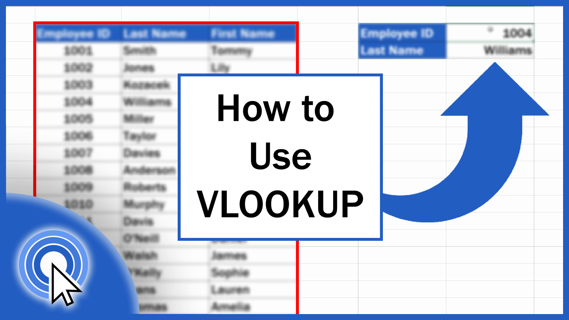
Let’s break it down. VLOOKUP is a function in Excel that searches for a specific value in the leftmost column of a table and retrieves related information from another column in the same row. Think of it like looking up someone’s phone number in a contact list. You know the person’s name, and you want to find their number. VLOOKUP does the same thing but with any type of data you throw at it.

For example, say you have a list of employees and their departments. If you want to find out which department a particular employee belongs to, VLOOKUP can do that in a snap. All you need is the employee’s ID or name, and VLOOKUP will fetch the corresponding department details. Pretty cool, right?

How to Use Vlookup - Where Do I Begin?

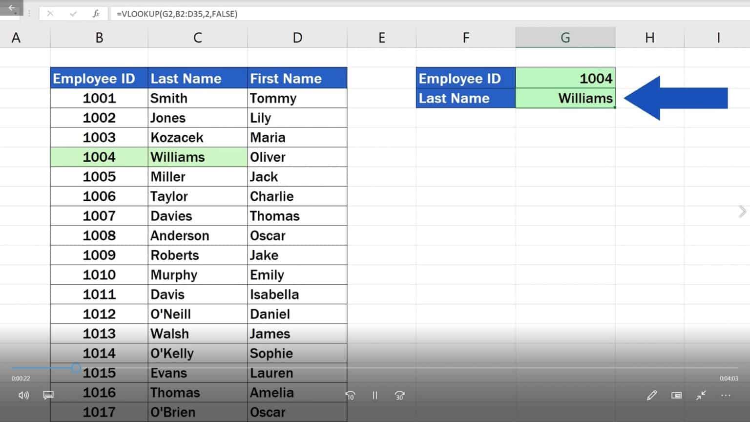
First things first, you need to know the basic structure of the VLOOKUP function. It looks like this: =VLOOKUP(lookup_value, table_array, col_index_num, [range_lookup]). Each part of this formula plays a role in finding the data you need. Let’s take a closer look at what each part means:

Lookup_value: This is the value you’re searching for. It could be a name, an ID, or any unique identifier.
Table_array: This is the range of cells where your data lives. Make sure your lookup value is in the first column of this range.
Col_index_num: This tells VLOOKUP which column to pull the data from. If you want data from the second column, you’d enter the number 2 here.
Range_lookup: This is optional but useful. You can set it to TRUE for approximate matches or FALSE for exact matches.

Why Would I Need to Know How to Use Vlookup?

Here’s the thing: VLOOKUP saves time. A lot of time. Instead of manually searching through hundreds or even thousands of rows, VLOOKUP does the heavy lifting for you. It’s like having a personal assistant who knows exactly where everything is. Plus, it reduces errors. When you’re working with large datasets, it’s easy to miss something or make a mistake. VLOOKUP ensures you get accurate results every time.

Now, let’s talk about real-world scenarios. Say you’re managing a team and need to track everyone’s performance metrics. With VLOOKUP, you can easily pull up each person’s data without breaking a sweat. Or maybe you’re organizing a school event and need to check which students are signed up for which activities. VLOOKUP makes this process a breeze.

How Can I Avoid Common Vlookup Errors?

Even the best of us make mistakes sometimes, but with VLOOKUP, a little preparation goes a long way. One common issue is when the lookup value isn’t in the first column of your table. Remember, VLOOKUP always starts its search in the leftmost column. If your data isn’t set up this way, consider rearranging it or using a different function, like INDEX and MATCH.

Another frequent problem is mismatched data types. For instance, if your lookup value is a number but the data in your table is stored as text, VLOOKUP won’t find a match. To avoid this, ensure that both your lookup value and the data in your table are in the same format. Lastly, double-check your column index number. Entering the wrong number could lead to pulling data from the wrong column.

How to Use Vlookup with Exact Matches

Exact matches are what most people use VLOOKUP for. Let’s say you have a list of products and their prices. If you want to find the price of a specific product, you’d use an exact match. To do this, simply set the range_lookup argument to FALSE. This tells VLOOKUP to only return results that exactly match your lookup value.

For example, if you’re looking for the price of an apple in a table, your formula might look like this: =VLOOKUP("apple", A2:C10, 2, FALSE). This searches for the word “apple” in column A and returns the corresponding value from column B.

What If My Data Isn’t Perfectly Aligned?

Not all data is perfectly organized, and that’s okay. Sometimes the value you’re searching for isn’t in the leftmost column. In these cases, you can’t use VLOOKUP directly. Instead, you can combine the INDEX and MATCH functions to achieve the same result. This might sound a bit tricky, but it’s actually quite straightforward once you get the hang of it.

For instance, if you’re searching for “Chicago” in a list of cities but it’s not in the first column, you’d use the MATCH function to find its position and then use INDEX to retrieve the related information. It’s a bit more work, but it gets the job done.

How Do Wildcards Work in VLOOKUP?

Wildcards are like secret codes that help you find partial matches. The asterisk (*) stands for any number of characters, while the question mark (?) represents a single character. This comes in handy when you’re not sure about the exact value you’re looking for.

For example, if you’re searching for a product that starts with “banana,” you could use =VLOOKUP("banana*", A2:C10, 2, FALSE). This would return the price of any product that begins with “banana,” such as “banana bread” or “banana chips.”

How to Use Vlookup Across Multiple Sheets

Not all your data will live on the same sheet, and that’s where VLOOKUP’s versatility shines. You can use it to pull data from another sheet or even another workbook. Just reference the sheet name followed by an exclamation mark (!) before the table range.

For example, if your data is on a sheet named “Data,” your formula might look like this: =VLOOKUP("apple", Data!A2:C10, 2, FALSE). This searches for “apple” in column A of the “Data” sheet and returns the corresponding value from column B.

When Should I Use Approximate Matches?

Approximate matches are useful when you’re dealing with sorted data and want to find the closest match. For example, if you have a list of grades and you want to assign letter grades based on score ranges, you’d use an approximate match. To do this, set the range_lookup argument to TRUE.

For instance, if you’re looking for the grade corresponding to a score of 85, your formula might look like this: =VLOOKUP(85, A2:B10, 2, TRUE). This returns the grade for the closest score less than or equal to 85.

What Are Some Alternatives to VLOOKUP?

While VLOOKUP is great, it’s not the only tool in the box. Depending on your situation, other functions might be better suited to your needs. For example, INDEX and MATCH offer more flexibility and can handle cases where the lookup value isn’t in the first column. HLOOKUP works similarly to VLOOKUP but searches across rows instead of columns.

Ultimately, the choice depends on your specific requirements. Don’t be afraid to experiment and see what works best for you. After all, Excel is all about finding solutions that fit your unique challenges.

How to Use Vlookup with Dynamic Formulas

Dynamic formulas make your spreadsheets smarter by allowing you to update data automatically. Instead of hardcoding values into your formulas, you can use cell references to create dynamic lookups. This means that whenever you change the value in a cell, the formula updates automatically.

For example, if you want to find the price of a product based on user input, you could use a formula like =VLOOKUP(D1, A2:C10, 3, FALSE). Here, D1 contains the lookup value, so changing it updates the result instantly.

So, there you have it—a comprehensive guide to using VLOOKUP in Excel. From basic operations to advanced techniques, this function has something for everyone. Whether you’re a beginner or a seasoned pro, VLOOKUP can help you work smarter, not harder.

Summary of How to Use Vlookup

VLOOKUP is an essential tool for anyone who works with data in Excel. By understanding its basic structure and learning how to avoid common errors, you can harness its full potential. From exact matches to wildcards, from single sheets to multiple workbooks, VLOOKUP offers endless possibilities. So next time you’re faced with a mountain of data, remember: VLOOKUP is your trusty sidekick, ready to help you conquer it with ease.

How to Use the VLOOKUP Function in Excel (Step by Step)

Details

How to Use the VLOOKUP Function in Excel

Details

Detail Author:

Name : Lia Hand
Username : miracle09
Email : eichmann.domingo@mcglynn.com
Birthdate : 2005-05-13
Address : 3504 Alek Row West Ryleychester, AR 49127-5913
Phone : +1-859-653-4332
Company : Funk Group
Job : Appliance Repairer
Bio : At et harum ad et impedit est. Autem soluta omnis excepturi corrupti. Et assumenda quidem dolores perspiciatis dolorum.

Socials

facebook:

url : https://facebook.com/ronnyparisian
username : ronnyparisian
bio : Sint corrupti expedita eligendi earum adipisci asperiores dignissimos.
followers : 5445
following : 2433